Prepare input data

1. A mutaiton file.

This file contains mutations identified from a tumor type. This file must be tab delimited with 5 columns. The 5 columns are chr, position, reference allele, observed allele, other columns are optional and will be ignored. The column names shoud be as indicated in the following example file. In ‘chromosome’ column you can either add ‘chr’ or not. e.g. ‘chr1’ or just ‘1’ is fine.

We have provided an example mutation file with the software in the data\ folder. The example file looks like this:

Chromosome	Position	Ref	Alt	SampleID
1	100181217	C	T	TCGA-QN-A5NN-01A-11D-A28R-08
1	103352425	G	A	TCGA-QN-A5NN-01A-11D-A28R-08
1	103453188	C	A	TCGA-NG-A4VU-01A-11D-A28R-08
1	103470202	G	T	TCGA-N6-A4VE-01A-11D-A28R-08
1	104122106	C	A	TCGA-N5-A59F-01A-11D-A28R-08
1	104160643	C	A	TCGA-N9-A4Q1-01A-11D-A28R-08

Note: currently only hg19 coordinates are accepted for mutation files. If your mutation file is aligned to other genome build, you can use the LiftOver tool provided by UCSC.

2. Annotation files.

The annotations files list all possible mutations within sequenced regions and provide annotation for each mutation. For exome sequencing studies, you can use the annotations files provided with the software. They are in data/ folder. There are 9 such files under data/ folder for each of the 9 nucleotide change types defined as

• 1. C:G to G:C mutations at CpG dinucleotides
• 2. C:G to A:T mutations at CpG dinucleotides
• 3. C:G to T:A mutations at CpG dinucleotides
• 4. C:G to G:C mutations not in CpG dinucleotides
• 5. C:G to A:T mutations not in CpG dinucleotides
• 6. C:G to T:A mutations not in CpG dinucleotides
• 7. A:T to T:A mutations
• 8. A:T to C:G mutations
• 9. A:T to G:C mutations

Functional annotations included are LoF, conservation, SiFT prediction, phylop prediction, splicing effect, MutationAssessor prediction, etc. To generate your annotation files, please see advanced way to run driverMAPS below.

Run driverMAPS

Step 1: Activating the environment

To activate the maps environment, execute

conda activate maps

Step 2: Modify the config file.

Here is the default config file config.yaml included with the software:

# Directory to keep outputs. Note that this directory name must end
# with a backslash ("/").
outputdir:
        "output/"

# Directory to keep log files. Note that this directory name must end
# with a backslash ("/").
logdir:
        "output/logs/"

# Directory that keeps _annodata.txt files. Note that this directory
# name must end with a backslash ("/").
annodir:
        "data/"

# Tumor names, can be one or multiple.
tumornames:
        - "TCGA-UCS"
          
mutationfile:
        "data/{tumorname}_mutations.txt"

# --- advanced configuration ---
# If infer beta_f for functional features in SMM model.There are several modes: 'none', means do not infer from data and use predefined parameters. this is the default. 'MLE', means using maximum likelihood estiamtion using data from a single tumor type. 'MLE-ASH', means when you have many tumor types and want to jointly estimate beta_f.
Funcvinfer:
        'none'

# If infer tumor specific HMM, if not, predefined HMM parameters
# (averaged across 20 tumor types) will be used.
HMMinfer:
        false

# Directory holding predefined parameters as used in the paper. Note
# that this directory name must end with a backslash ("/").
paramdir:
        "param/"

# Location where the R scripts are found. Note that this directory
# name must end with a backslash ("/").
scriptdir:
        "scripts/"

# Run algorithm configuration and parameters.
runconfig:
        "scripts/R00_config.R"

In most cases, you only need to change outputdir, logdir, tumornames and mutationfile. For tumornames, you can put one or multiple tumor names, depending on how many mutation files you have. Under the default configuration, the script will run for each tumor type independently. For mutationfile, one should put the location of the mutation file here. {tumorname} here is a wildcard and will automatically replaced by each tumor names provided in tumornames.

Example: If you don’t modify anything in this config file, it will look for /data/TCGA-UCS_mutations.txt as the mutation file and will produce output files under output/ and log files under output/logs/.

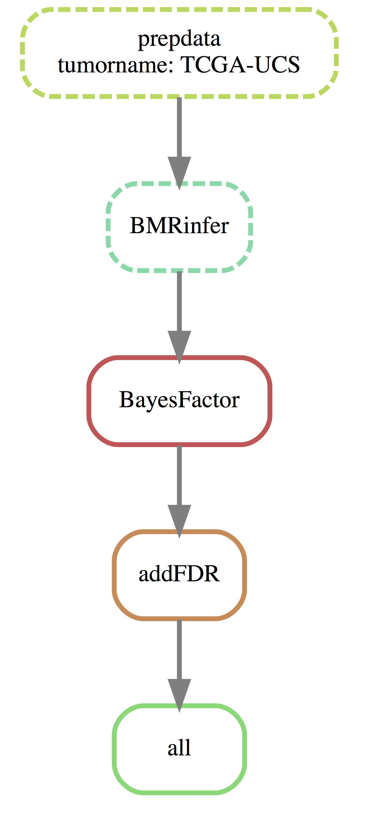
You can visualize the execution plan to verify if that’s your desired workflow:

cd path/to/workdir
snakemake -np --dag | dot -Tsvg > dag.svg

The dag.svg file will contain the execution plan. Here is the workflow plan generated based on the default config:

Step 3: Run driverMAPS

• Single-processor mode

The requirement (memory and time) for each step for one tumor type is given in the file cluster.json which is included in the software. The single processor mode takes around 10 hours to finish, requiring 12G memory.

You can run it interactively without submitting it to a computer cluster.

cd path/to/workdir
snakemake

To run it on a cluster, driverMAPS will submit jobs step by step onto your cluster based on configurations specified for each step in the cluster.json file. Run the following command (for SLURM systems):

cd path/to/workdir; snakemake -j 999 --cluster-config cluster.json --cluster "sbatch -n {cluster.n}  -t {cluster.time} --mem {cluster.mem} --job-name {cluster.name} --output {cluster.out} --error {cluster.err}"

Note: cluster.json provides configuration for each tumor type, so if you provided mutiple tumor names, the program will submit multiple jobs (one for each tumor), each following the configurations described in cluster.json and will run in parallel. Please modify the ’cluster.json` file and submitting command to fit the cluster system you are using.

• Multiple-processor mode

To increase speed, we have provided the parallel computing option and the run time can be significantly reduced. When using less than or equal to 4 cores, please allocate at least 12G memory. When using more than 4 cores, give an extra 3G memory for each additional core you requested. When using 4 cores, the run time is around 3-4 hours, when using 6 cores, the run time is around 2-3 hours.

To run driverMAPS using multiple cores, use the following command (for example using 10 cores):

cd path/to/workdir; snakemake --cores 10

Step 4: About rerun and exit You can hit crtl + C to terminate the run, however, this will not terminate jobs submitted to cluster. If your run failed at certain step, you can rerun the program and it will pick up from the step where it stops in the last run.

Step 5: Reading the results The main results are given in the following file: xxx_BayesFactorFDR.txt. Example output file:

gene	No_nonsyn	functypecode8	mycons	sift	phylop100	MA	No_unique_mutation	TSG_BF	OG_BF	Expected_syn	No_syn	BF	predtag	Posterior	FDR
PIK3CA	20	0	20	2	19	7	13	14.99481	83.74050	0.0539501	0	83.04735	OG	0.00e+00	0.0e+00
TP53	46	7	38	40	34	39	34	68.13620	62.31167	0.0177879	0	67.44600	TSG	0.00e+00	0.0e+00
FBXW7	21	1	21	20	18	13	14	25.79546	55.67678	0.0371409	0	54.98364	OG	0.00e+00	0.0e+00
KRAS	7	0	7	7	7	7	4	10.09354	51.96083	0.0089269	0	51.26768	OG	0.00e+00	0.0e+00
PPP2R1A	15	0	15	14	10	14	10	18.45914	48.93329	0.0658627	0	48.24014	OG	0.00e+00	0.0e+00
PTEN	10	4	9	0	8	6	10	15.33542	10.90877	0.0155942	0	14.65416	TSG	3.46e-05	5.8e-06

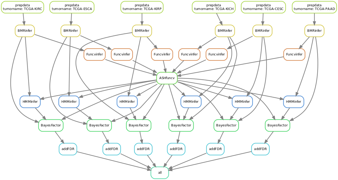
Reproduce results of running driverMAPS on real data.

This relates to Figure 4 of the paper.

Step 1: Download the mutation datasets

Download the mutation datasets for 20 tumor types from here

Step 2: Modify config file

Modify outputdir, logdir based on your needs. For tumornames, see below. Also modify Funcvinfer from “none” to “MLE-ASH”, modify HMMinfer from “false” to “true” (see below).

tumornames:
    - "TCGA-CESC"
    - "TCGA-PAAD"
    - "TCGA-ESCA"
    - "TCGA-KIRC"
    - "TCGA-KIRP"
    - "TCGA-KICH"
    - "TCGA-GBM"
    - "TCGA-LIHC"
    - "TCGA-UCS"
    - "TCGA-LUAD"
    - "TCGA-TGCT"
    - "TCGA-LUSC"
    - "TCGA-BLCA"
    - "TCGA-SARC"
    - "TCGA-HNSC"
    - "TCGA-CHOL"
    - "TCGA-PRAD"
    - "TCGA-BRCA"
    - "TCGA-UCEC"
    - "TCGA-SKCM"

Funcvinfer:
        'MLE-ASH'

HMMinfer:
        true

Modify mutationfile based on where you downloaded the mutation datasets.

Step 3: Run driverMAPS as previously described

It is suggested to use a computer cluster to run the above workflow

Step 4: Filter the results

driverMAPS is sensitive to false positive calls in sequencing data, because it will capture recurrent and clustered mutations as signs of positive selection, while in sequencing data such pattern can also be caused by false mapping/calling. Therefore, it is important to filter the identified significant genes by checking if mutations in these genes are false. One way to check is to manually go through the reads alignment plots for each of the mutations. We provide the blacklist file that was used in the paper to filter the gene lists here.

Reproduce results of running driverMAPS on simulated data.

This relates to Figure 3 of the paper.

Step 1: Download the simulated mutation datasets

Download the simulated mutation datasets of different sample sizes here.

Step 2: Modify config file

Modify outputdir, logdir in the config.yaml file based on your needs. For tumornames, HMMinfer and Funcvinfer give the following specifications:

tumornames:
        ["simulate_n100","simulate_n200","simulate_n400","simulate_n600","simulate_n800","simulate_n1000"
,"simulate_n1500","simulate_n2000"]

Funcvinfer:
        'MLE'

HMMinfer:
        true

Note in the paper, we also only used three of the functional covariates (LoF, conservation, MA) instead of five shown in Figure 2, so you will need to change the following code Funcvars <- c("functypecode", "mycons", "sift", "phylop100", "MA") in the scripts/R00_config.R file to Funcvars <- c("functypecode","mycons", "MA").

Step 3: Run driverMAPS as previously described

It is suggested to use a computer cluster to run the above workflow.